6.1 Interactive Plots using Plotly
- Here we will use the COVID-19 data provided by John Hopkins University
library(ggplot2)
library(maps)
library(ggthemes)
library(plotly)
library(scales)
library(dplyr)
library(tidyr)

# download data
d1 = read.csv("https://raw.githubusercontent.com/CSSEGISandData/COVID-19/master/csse_covid_19_data/csse_covid_19_time_series/time_series_covid19_confirmed_global.csv",
    check.names = FALSE)
# head(d1)- Data is in wide format let’s convert in long format for visualisation
# rename Provice/State and Country columns
colnames(d1)[1:2] = c("State", "Country")

d1.2 = pivot_longer(d1, cols = -c(State, Country, Lat, Long), names_to = "Date",
    values_to = "Cases")
# convert dates

d1.2$Date = as.Date(d1.2$Date, format = "%m/%e/%y")- Aggregate cases by day (dropping the state)
d2 = aggregate(d1.2$Cases, by = list(Lat = d1.2$Lat, Long = d1.2$Long, Country = d1.2$Country,
    Date = d1.2$Date), FUN = sum)
colnames(d2)[5] = "Cases"
# reorder
d2 = d2[, c(4, 1, 2, 3, 5)]- Let’s find top 10 by case numbers
- Using aggregate to find sum by country to find top 10
top1 = aggregate(d2$Cases, by = list(Date = d2$Date, Country = d2$Country), FUN = sum)
# select the last date to get overall total
top10 = top1[top1$Date == "2020-07-25", ]
# select top 10
top10 = top10[order(-top10$x), ][1:10, ]
# let's include Aus
top10_country = c(top10$Country, "Australia")- Use ggplot to create a line chart 6.1
colnames(top1)[3] = "Cases"
data_p = top1[top1$Country %in% c(as.character(top10_country)), ]

p1 = ggplot(data = data_p, aes(Date, log(Cases), color = Country, group = Country)) +
    geom_line(stat = "identity", size = 1) + scale_x_date(labels = date_format("%d/%m"),
    breaks = "7 days") + theme_wsj()
p1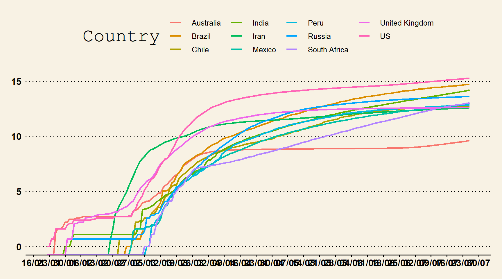
Figure 6.1: Line Chart with Custom Theme
- Create custom color vector and a line chart with basic theme to convert to plotly 6.2
myCol2 = c("slateblue1", "purple3", "turquoise2", "skyblue", "steelblue", "blue2",
    "navyblue", "orange", "tomato", "coral2", "palevioletred", "violetred", "red2",
    "springgreen2", "yellowgreen", "palegreen4", "wheat2", "tan", "tan2", "tan3",
    "brown", "grey70", "grey50", "grey30")

p2 = ggplot(data_p, aes(Date, Cases, group = Country, color = Country)) + geom_line(size = 1.5) +
    geom_point(size = 1.5) + scale_colour_manual(values = myCol2, "Countries") +
    geom_text(data = data_p[data_p$Date == max(data_p$Date), ], aes(x = as.Date(max(data_p$Date) +
        4), label = Country), hjust = -0.01, nudge_y = 0.01, show.legend = FALSE) +
    expand_limits(x = as.Date(c(min(data_p$Date), max(data_p$Date) + 5))) + scale_x_date(breaks = seq(as.Date(min(data_p$Date)),
    as.Date(max(data_p$Date) + 5), by = "7 days"), date_labels = "%m/%d") + scale_y_continuous(labels = comma) +
    theme_classic() + theme(axis.title = element_text(size = 15, face = "bold"))
p2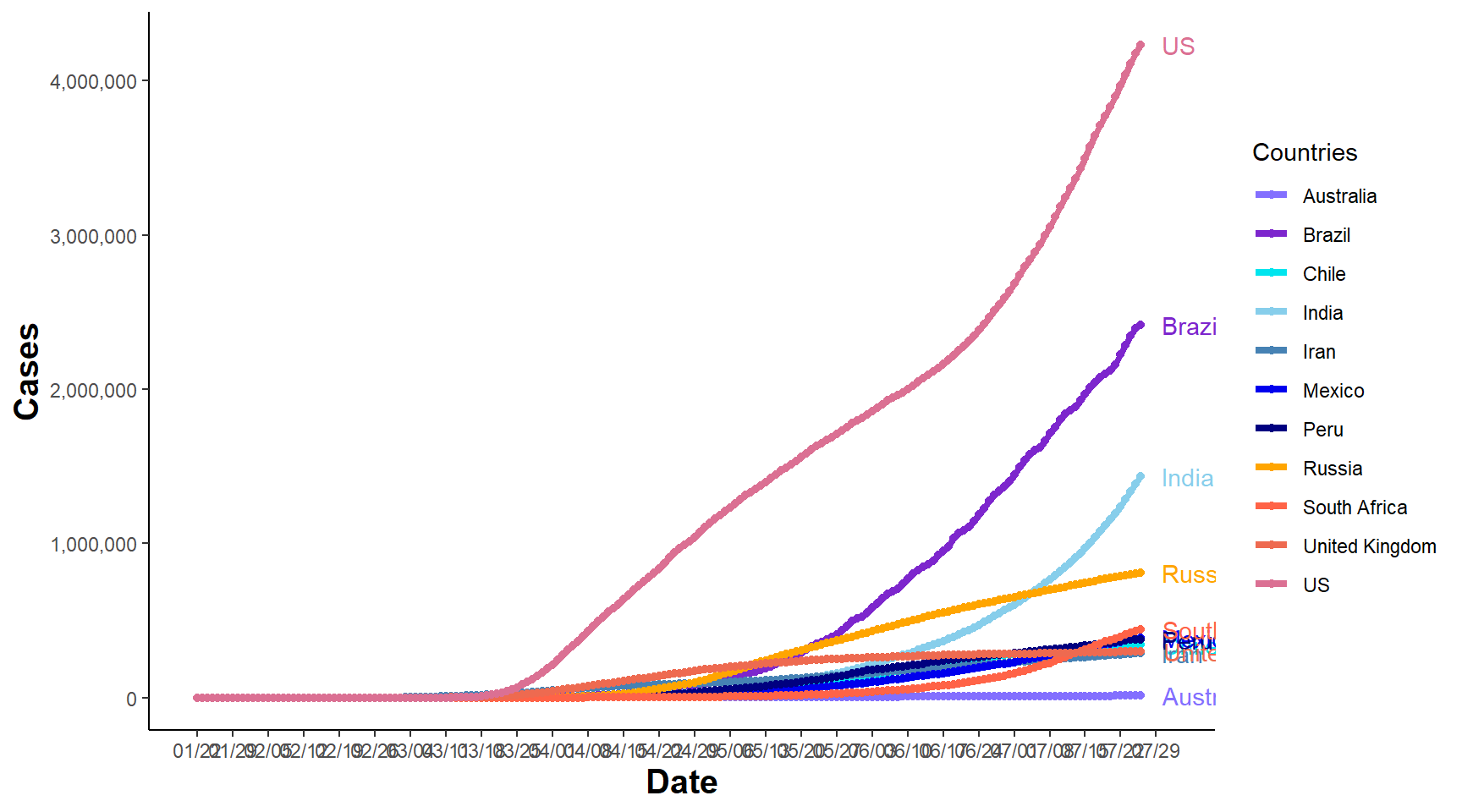
Figure 6.2: Line Chart
- Convert to plotly for interactive graphics 6.3
Figure 6.3: Interactive Line Chart