5.3 Introduction to ggplot2

• ggplot2 (Wickham 2009) is an R package which provides a large variety of plotting functionality to enable better and highly customisable graphs.
• These functions in ggplot2 are based on the grammar of graphics (Wickham 2010) which is a more formal and structured way to plotting, for a list of various possible graphs, customisation settings and procedures see https://ggplot2.tidyverse.org/

5.3.1 \(\mathtt{qplot}\)

• \(\mathtt{qplot}\) stands for quick plot and it makes is easy to produce plots which may often require several lines of codes using base R graphics system.

• \(\mathtt{qplot}\) is particularly useful for beginners as they are just getting used to the \(\mathtt{plot}\) function from the base package also the data arguments in \(\mathtt{qplot}\) are same as in the \(\mathtt{plot}\) function (see \(\mathtt{help(qplot)}\) for other arguments to the function).

x = rnorm(100)
y = rnorm(100)
# load the library
library(ggplot2)
# simple scatterplot using qplot
qplot(x, y)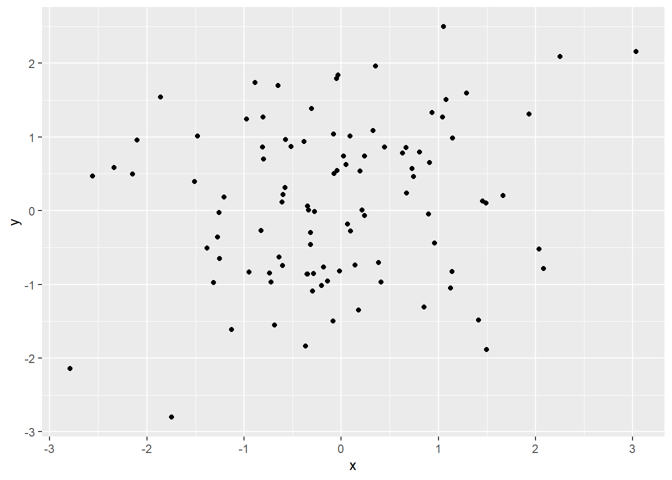

Figure 5.12: Scatterplot using qplot

• The argument geom, which stands for geometric objects drawn to represent data has to be changed to “line” create this line plot.

• Similarly there is an option to plot histograms using the argument geom=“histogram”

load("data/data_fin.RData")
# line plot using qplot
qplot(x = FinData$Date, y = FinData$DJI, geom = "line", xlab = "Dates", ylab = "Prices", 
    main = "DJIA Price Timeseries")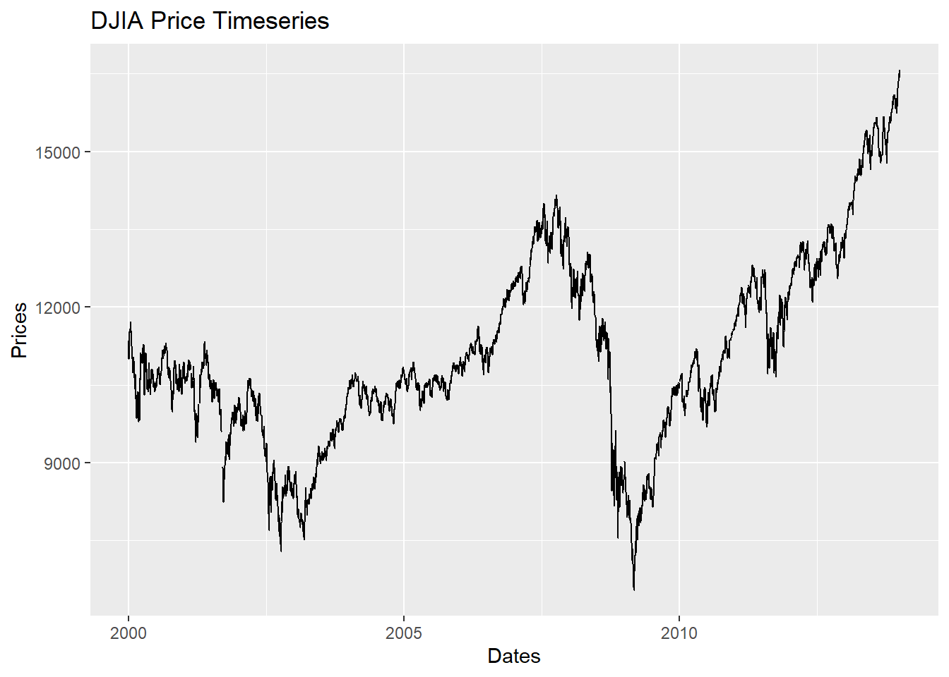

Figure 5.13: Line Plot with lables using qplot

5.3.2 Layered graphics using \(\mathtt{ggplot}\)

• The \(\mathtt{qplot}\) function is just sufficient for creating various plots with better presentation compared to base R plots but the true capabilities of ggplot2 are realised by the function \(\mathtt{ggplot}\).

• It is important to note that \(\mathtt{ggplot}\) function requires the data in “long” format and hence it is required to first transform the dataset to “long” from “wide” format as in ggplot2, groups are identified by rows, not by columns.

# Read 'long' format data
load("data/GDP_l.RData")
# data snapshot
head(GDP_l)

  Year   Country      GDP
1 1990 Australia 18247.39
2 1991 Australia 18837.19
3 1992 Australia 18599.00
4 1993 Australia 17658.08
5 1994 Australia 18080.70
6 1995 Australia 20375.30

# creating the aesthetics using ggplot
p1 = ggplot(GDP_l, aes(Country, GDP, fill = Year))

• A plot can be created by adding another layer to p1

# figure
p1 + geom_bar(stat = "identity")

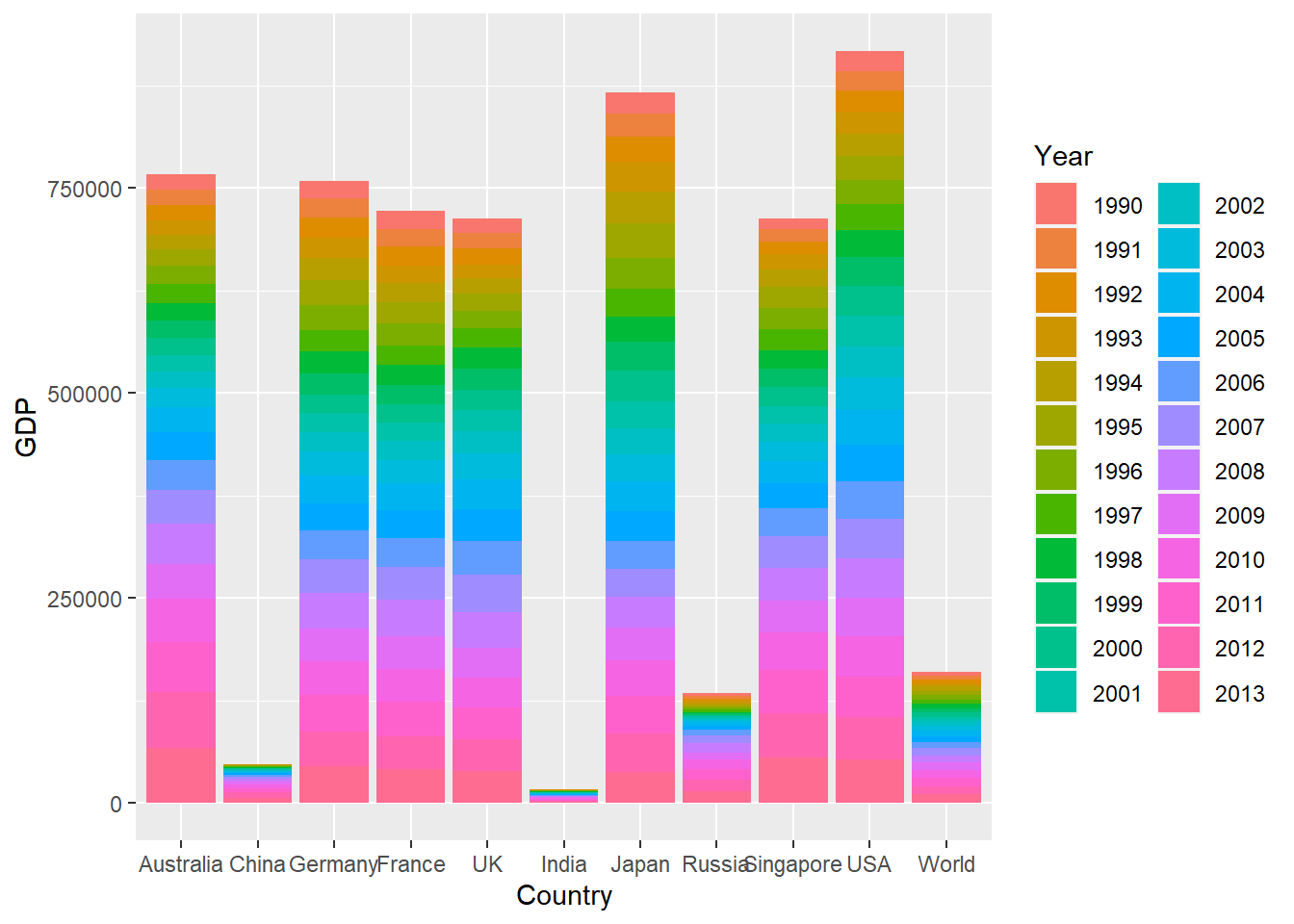
Figure 5.14: Bar Chart Using ggplot function

• To draw a line chart using \(\mathtt{ggplot}\), \(\mathtt{geom\_line()}\)

# change the aesthetics to show time on X-axis and GDP values on Y-axis the
# colour line fill be according to the country
p2 = ggplot(GDP_l, aes(Year, GDP, colour = Country, group = Country))
p2 + geom_line()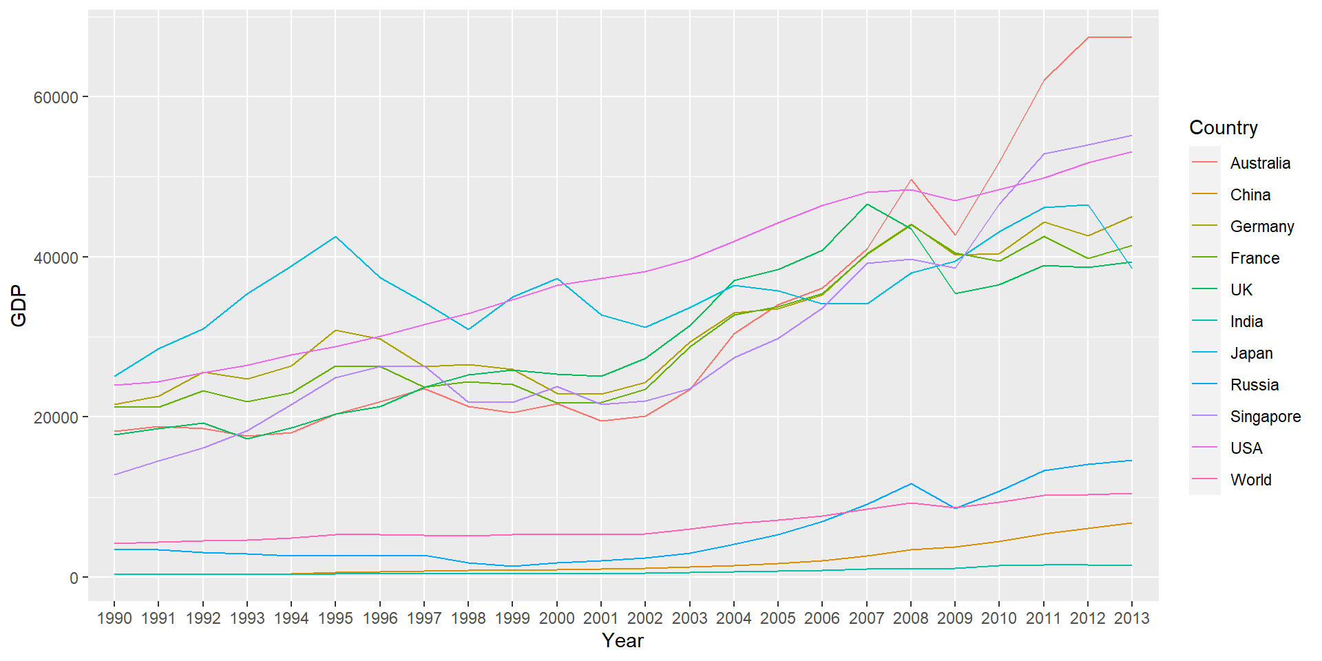

Figure 5.15: Line Chart Using ggplot

• These lines can also be drawn in separate panels using faceting. Faceting creates a subplot for each group side by side.

• Faceting can be used to either to split the data into vertical groups using \(\mathtt{facet\_grid}\) or horizontal groups using \(\mathtt{facet\_wrap}\).

• Figure plots GDP for each country in a separate subplot using grid faceting.

# change the aesthetics to show time on X-axis and GDP values on Y-axis the
# colour line fill be according to the country
p2 = ggplot(GDP_l, aes(Year, GDP, colour = Country, group = Country))
p2 + geom_line() + facet_grid(Country ~ .)

Figure 5.16: Faceting in ggplot (Line Chart)

5.3.3 Arranging plots using gridExtra

• There are a few pacakges which allow to arrange ggplots in a grid or a speacific order. gridExtra is one of them and is quite useful in arranging the plots.

• Look at the Vignette for egg package for more options. https://cran.r-project.org/web/packages/egg/vignettes/Ecosystem.html

• Let’s create three ggplots

p1.1 = ggplot(GDP_l, aes(x = Year, y = GDP))
p2.1 = p1.1 + geom_bar(aes(fill = Country), stat = "identity", position = "dodge")

• Stacked bar chart (previous example)

p1.2 = ggplot(GDP_l[GDP_l$Country %in% c("Australia", "UK", "USA"), ], aes(Year, 
    GDP))
p2.2 = p1.2 + geom_col(aes(fill = Country)) + labs(title = "GDP for Aus, US and UK")  #using labs to modify title
p2.2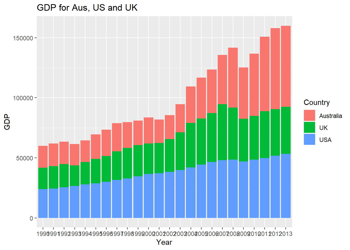

Figure 5.17: Bar Chart with Selected Data

• Stock data

p1.3 = ggplot(FinData, aes(x = Date, y = DJI))
p2.3 = p1.3 + geom_path(colour = "darkblue") + geom_smooth(colour = "black") + theme_linedraw()  #changing theme
p2.3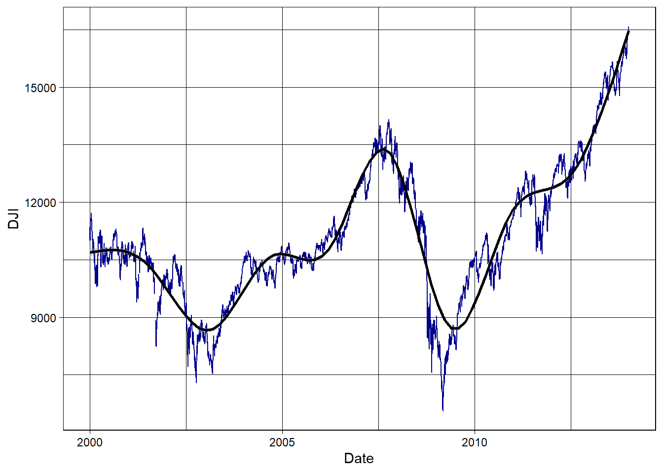

Figure 5.18: Stock Series Plot with Smooth Curve

• Now use gridExtra to put these together

library(gridExtra)
fig1 = grid.arrange(p2.1, p2.2, p2.3, nrow = 3, heights = c(20, 12, 12), top = "Combined plots in three rows")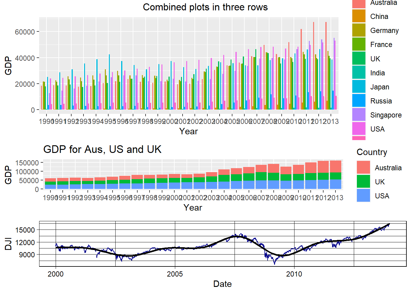

Figure 5.19: Combined plots

• The plots can be saved using the \(\mathtt{ggsave}\) function

ggsave(filename = "combined_plot.pdf", plot = fig1)

References

Wickham, Hadley. 2009. Ggplot2: Elegant Graphics for Data Analysis. Springer.

Wickham, Hadley. 2010. “A Layered Grammar of Graphics.” Journal of Computational and Graphical Statistics 19 (1): 3–28.